2018年12月7日:习题讲解
第九章
习题9.4
【题目】:
使用数据集Growth.dta考察贸易与增长的关系,该数据集的被解释变量为65个国家1960——1995年的平均增长率,而主要解释变量为1960——1995年的平均贸易开放度(tradeshare)。
(1)将growth与tradeshare的散点图和线性拟合图画在一起。二者看起来是否有关系?
(2)有一个国家马耳他(Malta),其贸易开放度比其他国家高很多,在散点图上找出马耳他。它是否像极端值?
(3)使用全样本,把growth对tradeshare进行回归,该回归的斜率和截距的估计值分别是多少?
(4)计算每个观测值的影响力,以及此影响力的最大值和平均值只比,是否存在极端值?
(5)去掉马耳他重复上述回归,并再次回答(3)中的问题。
(6)马耳他在哪?马耳他的贸易开放度为什么这么高?是否应该在本研究中去掉马耳他?
(7)把growth对tradeshare,rgdp60(1960年的人均GDP),yearsschool(1960年的平均受教育年限),rev_coups(1960年-1995年的年平均政变次数),以及assassinations(1960——1995年的年平均政治暗杀次数)进行回归。评论各变量系数的符号、统计显著性及经济意义。
(8)为什么把变量r60与yearsschool的取值定为起初的1960年?
【解答】:
(1):散点图&线性拟合图
use growth, clear
tw ///
lfit growth tradeshare || ///
sc growth tradeshare ||, ///
leg(order(1 "线性拟合值") pos(1) ring(0) row(1)) ///
xti("1960——1995年的平均贸易开放程度") ///
yti("1960——1995年的平均增长率") ///
xlab(, format(%6.0f))
gr export "9_4散点+线性拟合图.png", replace
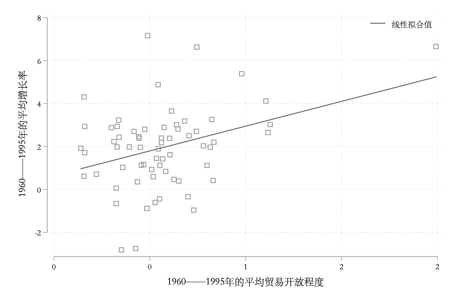
显然,贸易开放程度和经济增长之间存在正相关的关系。
(2):马耳他
* 预保存数据
preserve
keep if country_name == "Malta"
* 存储马耳他的数据
local y = growth[1]
local x = tradeshare[1]
di "x = " `x' " 而 y = "`y'
* 恢复数据
restore
* 可以看到local变量还在
di "x = " `x' " 而 y = "`y'

tw ///
lfit growth tradeshare || ///
scatteri `y' `x' (7) "马耳他", ms(D) mc("dkorange") || ///
sc growth tradeshare if country_name != "Malta" ||, ///
leg(order(1 "线性拟合值") pos(1) ring(0) row(1)) ///
xti("1960——1995年的平均贸易开放程度") ///
yti("1960——1995年的平均增长率") ///
xlab(, format(%6.0f))
gr export "9_4散点+线性拟合图+极端值.png", replace
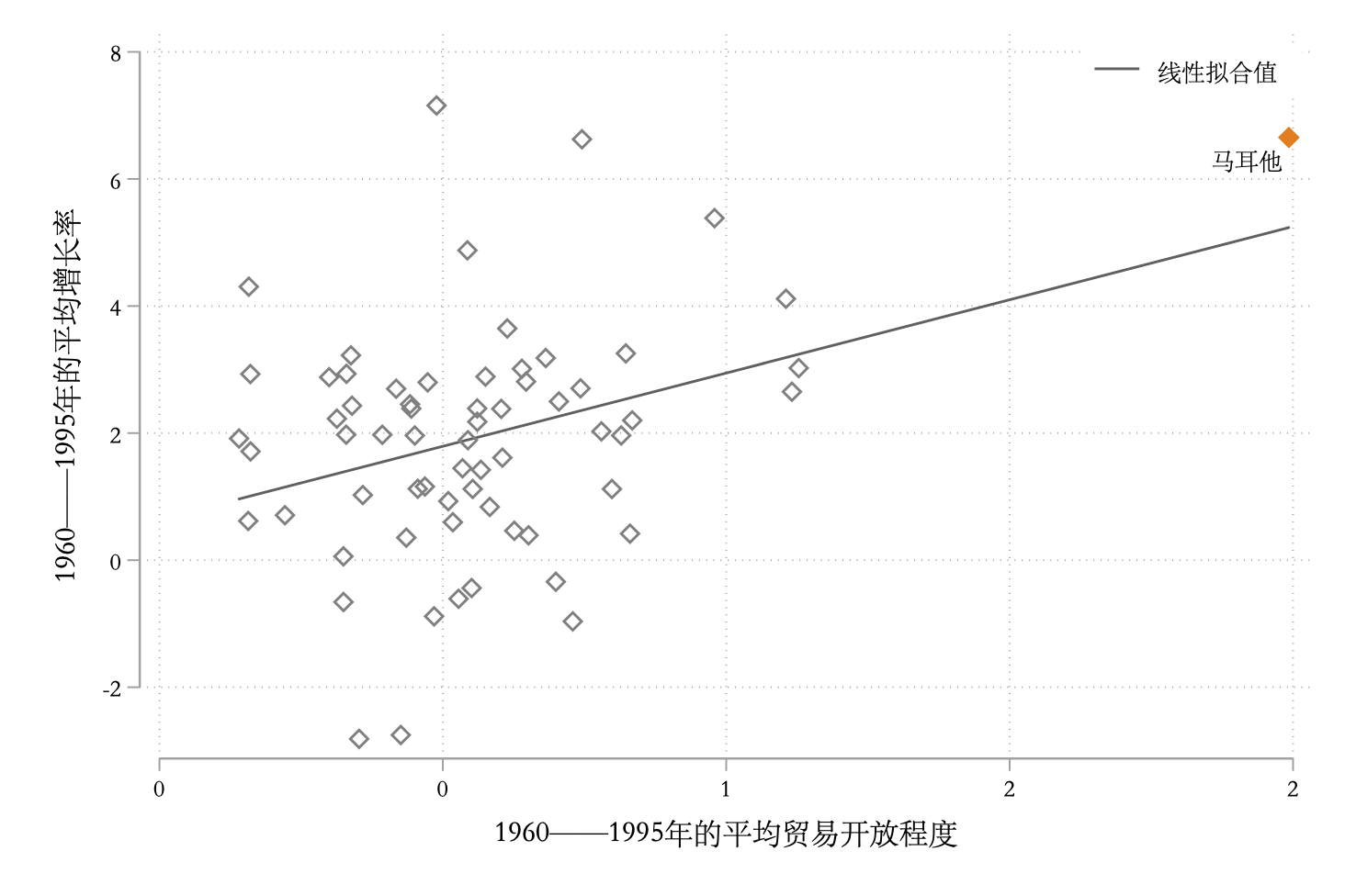
可以看出,马耳他看起来很像极端值。
(3):全样本回归
. reg growth tradeshare

      Source |       SS           df       MS      Number of obs   =        65
-------------+----------------------------------   F(1, 63)        =      8.89
       Model |  28.4885066         1  28.4885066   Prob > F        =    0.0041
    Residual |  201.851551        63  3.20399287   R-squared       =    0.1237
-------------+----------------------------------   Adj R-squared   =    0.1098
       Total |  230.340057        64  3.59906339   Root MSE        =      1.79

------------------------------------------------------------------------------
      growth |      Coef.   Std. Err.      t    P>|t|     [95% Conf. Interval]
-------------+----------------------------------------------------------------
  tradeshare |   2.306434    .773485     2.98   0.004     .7607473     3.85212
       _cons |   .6402653   .4899767     1.31   0.196    -.3388749    1.619405
------------------------------------------------------------------------------
斜率为2.3064,截距为0.6403。
(4):影响力
* 计算leverage
predict lev, lev
qui sum lev
di r(max)/r(mean)
计算的结果为12.87,经验规则表明,这是相当大的,因此认为存在极端值。
(5):去掉极端值的回归
. reg growth tradeshare if country_name != "Malta"

      Source |       SS           df       MS      Number of obs   =        64
-------------+----------------------------------   F(1, 62)        =      2.90
       Model |  9.28031557         1  9.28031557   Prob > F        =    0.0937
    Residual |  198.527844        62  3.20206201   R-squared       =    0.0447
-------------+----------------------------------   Adj R-squared   =    0.0292
       Total |   207.80816        63  3.29854222   Root MSE        =    1.7894

------------------------------------------------------------------------------
      growth |      Coef.   Std. Err.      t    P>|t|     [95% Conf. Interval]
-------------+----------------------------------------------------------------
  tradeshare |   1.680905   .9873624     1.70   0.094    -.2928046    3.654614
       _cons |   .9574107   .5803727     1.65   0.104    -.2027378    2.117559
------------------------------------------------------------------------------
此时斜率为1.6809,截距为0.9574。(对比刚刚的(2.3064和0.6403))
(6):马耳他
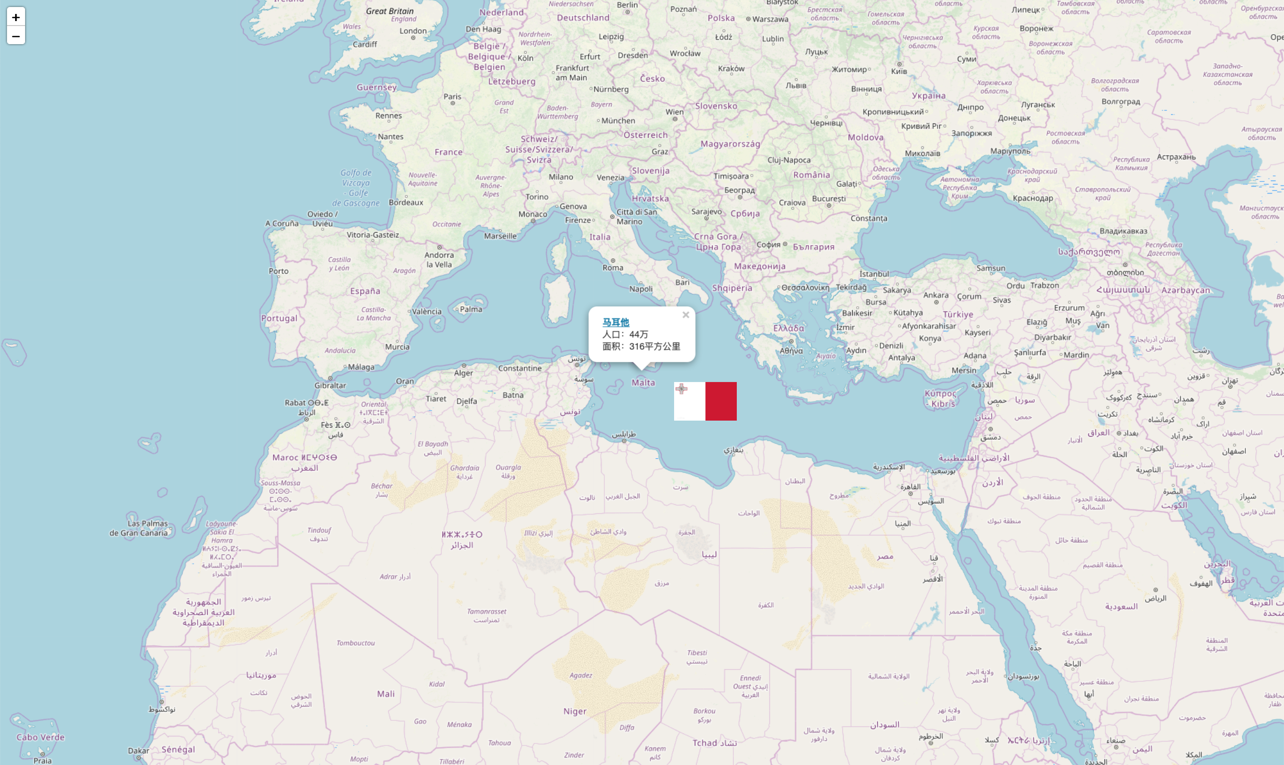
马耳他是一个位于地中海中心的岛国。是一个高度发达的资本主义国家,经济以服务业和金融业为主,旅游业是马耳他主要的外汇来源。马耳他同100多个国家和地区有贸易关系,欧盟是马耳他最重要的贸易伙伴。另外,马耳他社会保障体系较为完备,实行免费教育,免费医疗及退休保险制。
也就是地中海的这个位置:
绘图代码(R语言 + leaflet):
library(leaflet)

Maltatag <- makeIcon(
  iconUrl = "malta.jpeg",
  iconWidth = 90, iconHeight = 55,
  iconAnchorX = 22, iconAnchorY = 94
)
content <- paste(sep = "<br/>",
                 "<b><a href='https://baike.baidu.com/item/%E9%A9%AC%E8%80%B3%E4%BB%96'>马耳他</a></b>",
                 "人口:44万",
                 "面积:316平方公里"
)

leaflet() %>%
  setView(lng = 14.31, lat = 35.53, zoom = 5) %>%
  addTiles() %>%
  addPopups(lng = 14.31, lat = 36.5, content) %>%
  addMarkers(lng = 17.31, lat = 32.5, icon = Maltatag)
由于马耳他是极端值且对估计结果影响较大,所以还是去掉比较好。
(7):完整模型的估计
. reg growth tradeshare rgdp60 yearsschool rev_coups assasinations

      Source |       SS           df       MS      Number of obs   =        65
-------------+----------------------------------   F(5, 59)        =      6.61
       Model |  82.6634812         5  16.5326962   Prob > F        =    0.0001
    Residual |  147.676576        59  2.50299281   R-squared       =    0.3589
-------------+----------------------------------   Adj R-squared   =    0.3045
       Total |  230.340057        64  3.59906339   Root MSE        =    1.5821

-------------------------------------------------------------------------------
       growth |      Coef.   Std. Err.      t    P>|t|     [95% Conf. Interval]
--------------+----------------------------------------------------------------
   tradeshare |   1.561696   .7579475     2.06   0.044     .0450462    3.078345
       rgdp60 |  -.0004693   .0001482    -3.17   0.002    -.0007659   -.0001728
  yearsschool |   .5748461   .1393379     4.13   0.000     .2960316    .8536606
    rev_coups |  -2.157503   1.110292    -1.94   0.057    -4.379191    .0641853
assasinations |   .3540784   .4773943     0.74   0.461    -.6011854    1.309342
        _cons |   .4897603   .6895996     0.71   0.480    -.8901254    1.869646
-------------------------------------------------------------------------------
- tradeshare:符号为正,在5%的显著性水平上显著,表示平均贸易开放程度每增加一个单位,经济平均增长率平均上升1.56%。
- rgdp60:符号为负,在5%的显著性水平上显著,表示1960年的人均GDP每增加一块钱,经济平均增长率就平均下降0.00047%。
- yearsschool:符号为正,在5%的显著性水平上显著,表示1960年的平均受教育年限每增加1年,经济平均增长率就平均上升0.57%。
- rev_coups:符号为负,在10%的显著性水平上显著,表示1960——1995年间的年平均政变次数每增加一次,经济平均增长率就平均下降2.15%。
- assassinations:符号为负,但是很不显著,因此没有意义。
(8):期初
这样可以避免逆向因果的问题,而且比较符合逻辑。
习题9.5
【题目】:
美国的汽油需求函数是否稳定?使用数据集gasoline.dta,估计美国1953——2004年的汽油需求函数(参见第八章):
其中被解释变量lgasq为人均汽油消费量的对数,解释变量lincome为人均收入对数,lgasp为汽油价格指数的对数,lpnc为新车价格指数的对数,lpuc为二手车价格指数的对数。
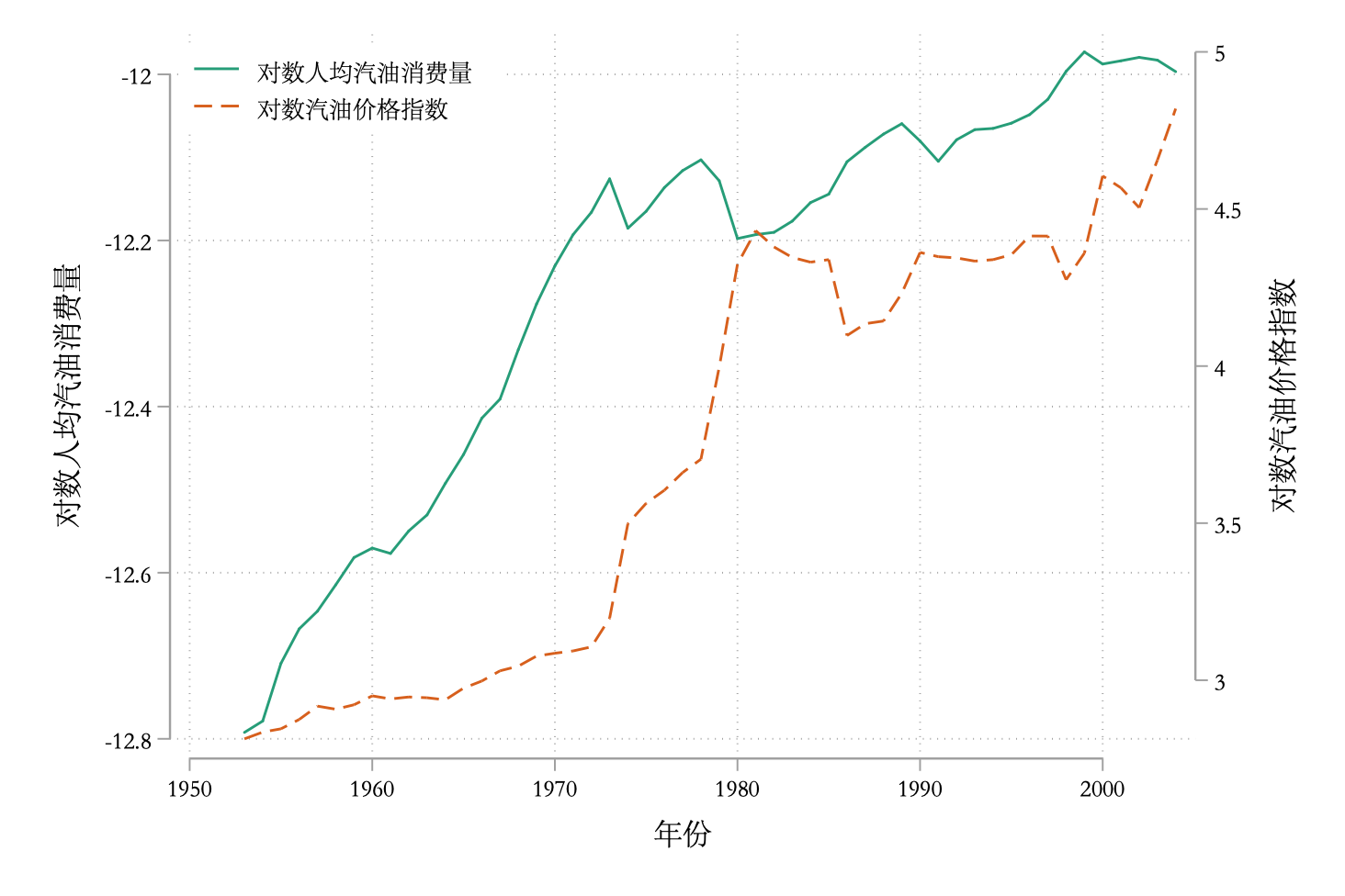
(1)将lgasq与lgasp的时间趋势图画在一起。根据此图,在1953——2004年期间,美国的汽油需求函数是否曾出现结构变动?
(2)使用OLS估计方程(9.48).
(3)使用BP检验与怀特检验,检验是否存在异方差。
(4)使用BG检验与Q检验,检验是否存在自相关。
(5)1973年10月爆发石油危机,可能引发汽油需求的结构变动。使用虚拟变量法,检验美国的汽油需求函数是否在1974年发生结构变动。根据(3)与(4)的检验结果决定是否应该使用稳健标准误。
【解答】:
(1):时间趋势图
use gasoline, clear
* 使用调色板命令配色
colorscheme 3, palette(Dark2)
ret list
* "027 158 119" "217 095 002"
tw ///
line lgasq year, lc("027 158 119") yaxis(1) || ///
line lgasp year, lc("217 095 002") yaxis(2) ||, ///
leg(order(1 "对数人均汽油消费量" 2 "对数汽油价格指数") pos(10) ring(0)) ///
yti("对数人均汽油消费量", axis(1)) ///
yti("对数汽油价格指数", axis(2)) ///
xti("年份")

gr export "9_5趋势图.png", replace
(2):OLS估计
. reg lgasq l.lgasq lincome lgasp lpnc lpuc

      Source |       SS           df       MS      Number of obs   =        51
-------------+----------------------------------   F(5, 45)        =   1830.77
       Model |  2.59056415         5   .51811283   Prob > F        =    0.0000
    Residual |  .012735088        45  .000283002   R-squared       =    0.9951
-------------+----------------------------------   Adj R-squared   =    0.9946
       Total |  2.60329924        50  .052065985   Root MSE        =    .01682

------------------------------------------------------------------------------
       lgasq |      Coef.   Std. Err.      t    P>|t|     [95% Conf. Interval]
-------------+----------------------------------------------------------------
       lgasq |
         L1. |   .8309713   .0457633    18.16   0.000     .7387994    .9231433
             |
     lincome |   .1640462   .0550263     2.98   0.005     .0532175    .2748748
       lgasp |  -.0695317   .0147326    -4.72   0.000    -.0992047   -.0398587
        lpnc |  -.1783946   .0551726    -3.23   0.002    -.2895179   -.0672714
        lpuc |   .1270093   .0357704     3.55   0.001      .054964    .1990546
       _cons |   -3.12318   .9958266    -3.14   0.003    -5.128878   -1.117483
------------------------------------------------------------------------------
拟合的模型为:
(3):异方差检验
. estat hettest, iid

Breusch-Pagan / Cook-Weisberg test for heteroskedasticity
         Ho: Constant variance
         Variables: fitted values of lgasq

         chi2(1)      =     0.31
         Prob > chi2  =   0.5788

. estat hettest, iid rhs

Breusch-Pagan / Cook-Weisberg test for heteroskedasticity
         Ho: Constant variance
         Variables: L.lgasq lincome lgasp lpnc lpuc

         chi2(5)      =     7.46
         Prob > chi2  =   0.1884

. estat imtest, white

White's test for Ho: homoskedasticity
         against Ha: unrestricted heteroskedasticity

         chi2(20)     =     33.20
         Prob > chi2  =    0.0321

Cameron & Trivedi's decomposition of IM-test

---------------------------------------------------
              Source |       chi2     df      p
---------------------+-----------------------------
  Heteroskedasticity |      33.20     20    0.0321
            Skewness |       9.58      5    0.0881
            Kurtosis |       0.61      1    0.4356
---------------------+-----------------------------
               Total |      43.38     26    0.0176
---------------------------------------------------
两种BP检验的结果表明无法拒绝同方差的原假设,而怀特检验表明拒绝同方差的原假设。考虑到两种检验的区别,所以结论是:不存在线性的异方差,但是存在非线性的异方差。
(4):自相关检验
. tsset year
        time variable:  year, 1953 to 2004
                delta:  1 unit

. qui reg lgasq l.lgasq lincome lgasp lpnc lpuc

. * BG检验

. estat bgo

Breusch-Godfrey LM test for autocorrelation
---------------------------------------------------------------------------
    lags(p)  |          chi2               df                 Prob > chi2
-------------+-------------------------------------------------------------
       1     |          0.545               1                   0.4603
---------------------------------------------------------------------------
                        H0: no serial correlation

. estat bgo, nom

Breusch-Godfrey LM test for autocorrelation
---------------------------------------------------------------------------
    lags(p)  |          chi2               df                 Prob > chi2
-------------+-------------------------------------------------------------
       1     |          1.361               1                   0.2434
---------------------------------------------------------------------------
                        H0: no serial correlation

.
. * Q检验

. predict e1, r
(1 missing value generated)

. wntestq e1

Portmanteau test for white noise
---------------------------------------
 Portmanteau (Q) statistic =    25.2413
 Prob > chi2(23)           =     0.3380
两种检验都无法拒绝无自相关的原假设。
(5):检验结构变动
use gasoline, clear
gen yearid = (year >= 1973)
gen interaction = yearid * lgasp
reg lgasq l.lgasq lincome lgasp lpnc lpuc yearid interaction, r
结果:
Linear regression                               Number of obs     =         51
                                                F(7, 43)          =    2328.20
                                                Prob > F          =     0.0000
                                                R-squared         =     0.9967
                                                Root MSE          =     .01421

------------------------------------------------------------------------------
             |               Robust
       lgasq |      Coef.   Std. Err.      t    P>|t|     [95% Conf. Interval]
-------------+----------------------------------------------------------------
       lgasq |
         L1. |   .4682407    .096862     4.83   0.000     .2728999    .6635815
             |
     lincome |   .3143699   .0528124     5.95   0.000     .2078636    .4208762
       lgasp |   .5230541   .1386092     3.77   0.000      .243522    .8025862
        lpnc |  -.0353864   .0503548    -0.70   0.486    -.1369365    .0661638
        lpuc |   .0381906   .0297671     1.28   0.206    -.0218405    .0982217
      yearid |   1.934971     .42312     4.57   0.000     1.081668    2.788274
 interaction |  -.6175106   .1377708    -4.48   0.000    -.8953518   -.3396694
       _cons |  -11.08808   2.034093    -5.45   0.000    -15.19022   -6.985939
------------------------------------------------------------------------------

* 另外再进行检验
. test yearid interaction

 ( 1)  yearid = 0
 ( 2)  interaction = 0

       F(  2,    43) =   18.80
            Prob > F =    0.0000
由于存在异方差问题,所以使用稳健的标准误。
可以看出生成的虚拟变量和虚拟变量与汽油价格指数对数的交互项的系数都非常显著,因此认为在1973年发生了结构变动。